Variational Dequantization
In this post I’ll discuss methods for dequantizing discrete values for continuous distributions. We’ll start with why dequantization is needed, then move on to a simple method for the problem, and end with a more flexible and general method recently proposed in the Flow++ paper [1].
Most measurements in the real world are continuous, and therefore we may want to use a continuous distribution to model them. However, for the sake of storage, most measurement values are clipped to a pre-defined discrete set of values (aka. quantized). For instance, we typicall quantize images to an 8-bit integer in the range $[0, 255]$.
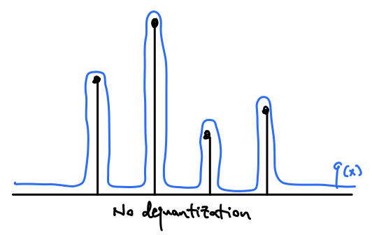
If we naively fit a continuous distribution to these quantized values, the model can learn to achieve high lihelihood by placing large spikes at these quantized values, while making the likelihood low everywhere else. This is an unnatural distribution that is unlikely to appear in the real world, and we would like to discourage our model from overfitting to the quantization. For the sake of simplicity, let’s assume our data is images, and has been quantized to the $[0, 255]$ in increments of 1.
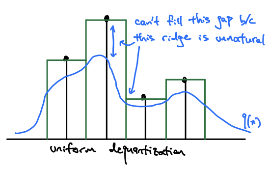
What might we do to prevent these spikes at the quantization centers? You might intuitively think to add some noise to smooth the values. $u \sim Uniform(0, 1)$ seems like a decent choice, since we just “fill” those quantization buckets equally. This is in fact the most common approach to dequantize discrete values for a continuous distribution [2]. However, this approach introduces flat step-wise regions into the data distribution, and while it’s better than having spikes, it is also unnatural and difficult to fit most parametric distributions.
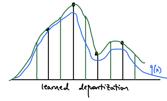
How do we improve this? We still want to add some smoothing noise $u$, but we don’t want it to be uniform noise around the quantization centers. So let’s make it a distribution that is dependent on what the value of $x$ is, and let’s learn that distribution, $u \sim r(u|x)$.
In order to learn $r(u|x)$, we need a loss function. It turns out the “hack” of adding quantization noise, learned or not, upper bounds the continuous data likelihood by the discrete data likelihood.
We want to learn a continuous distribution $q(x)$ for the data. Since the data we have are actually discrete and quantized, let’s say $q$ integrated over the quantization bin gives you the discrete distribution:
$$ Q(x) = \int_{[0, 1)} q(x+u) du $$
Let’s define $P(x)$ as the discrete, quantized data distribution that we are trying to fit. The discrete maximum likelihood estiamtor is $ \mathop{\mathbb{E}}_{x \sim P(x)}[Q(X)] $
$$
\begin{aligned}
\mathop{\mathbb{E}}{x \sim P(x)}[Q(X)]
&= \mathop{\mathbb{E}}{x \sim P(x)}\left[\log \int_{[0, 1)} q(x+u) du\right] \\
&= \mathop{\mathbb{E}}_{x \sim P(x)}\left[\log \int_{[0, 1)} r(u|x) \frac{q(x+u)}{r(u|x)} du\right] \\
&= \mathop{\mathbb{E}}_{x \sim P(x)}\left[\log \mathop{\mathbb{E}}_{u \sim r(u|x)} \left[\frac{q(x+u)}{r(u|x)} \right]\right] \\
&\ge \mathop{\mathbb{E}}_{x \sim P(x)}\mathop{\mathbb{E}}_{u \sim r(u|x)} \left[\log \frac{q(x+u)}{r(u|x)} \right] \\
&= \mathop{\mathbb{E}}_{x \sim P(x)}\mathop{\mathbb{E}}_{u \sim r(u|x)} \left[\log q(x+u) - \log r(u|x) \right]
\end{aligned}
$$
What we’ve done here is introduced a variational distribution to model the noise. If we use a flow for $r(u|x)$, we can train the model and dequantizer together using the path-wise gradient estiamtor, or the “reparameterization trick” as it’s known in VAEs. Note that the using uniform noise to dequantize is simply choosing the uniform distribution to be $r$.
By jointly training the noise distribution model and the data distribution model, we can find a dequantization method that is both a valid upper bound for the likelihood and is more natural for the data distribution to fit to.